
Magnetostatic
Algorithms for solving the 2D and 3D linear magnetostatic equations.
Problem
Solve:
$ \displaystyle{todo} $
Variational form
$ \displaystyle{ \int_{\Omega}{\frac{1}{\mu}\nabla\times\mathbf{A}\cdot\nabla\times\mathbf{AA}} - \int_{\Omega}{\mathbf{J}\cdot\mathbf{AA}} = 0 } $
Algorithms
2D
//Parameters
real Mu0 = 4.*pi*1.e-7; //Vacuum magnetic permeability
real MuC = 1.25e-6; //Copper magnetic permeability
real J0 = 500.e4; //Current density

//Mesh
int nn = 25; //Mesh quality
real BoxRadius = 2.; //"Inifite" boundary
real MagnetHeight = 1.; //Magnet height
real MagnetInternalRadius = 0.1; //Magnet internal radius
real MagnetExternalRadius = 0.2; //Magnet external radius

int BoxWall = 10;

int nnL = max(2., BoxRadius*nn/2.);
border b1(t=0., 2.*pi){x=BoxRadius*cos(t); y=BoxRadius*sin(t); label=BoxWall;};

border b2(t=0., 1.){x=MagnetInternalRadius+(MagnetExternalRadius-MagnetInternalRadius)*t; y=-MagnetHeight/2.;};
border b3(t=0., 1.){x=MagnetExternalRadius; y=-MagnetHeight/2.+MagnetHeight*t;};
border b4(t=0., 1.){x=MagnetExternalRadius-(MagnetExternalRadius-MagnetInternalRadius)*t; y=MagnetHeight/2.;};
border b5(t=0., 1.){x=MagnetInternalRadius; y=MagnetHeight/2.-MagnetHeight*t;};

border b6(t=0., 1.){x=-MagnetInternalRadius-(MagnetExternalRadius-MagnetInternalRadius)*t; y=-MagnetHeight/2.;};
border b7(t=0., 1.){x=-MagnetExternalRadius; y=-MagnetHeight/2.+MagnetHeight*t;};
border b8(t=0., 1.){x=-MagnetExternalRadius+(MagnetExternalRadius-MagnetInternalRadius)*t; y=MagnetHeight/2.;};
border b9(t=0., 1.){x=-MagnetInternalRadius; y=MagnetHeight/2.-MagnetHeight*t;};

int nnH = max(2., 10.*nn*MagnetHeight);
int nnR = max(2., 10._nn_(MagnetExternalRadius-MagnetInternalRadius));
mesh Th = buildmesh(
b1(nnL) + b2(nnR) + b3(nnH) + b4(nnR) + b5(nnH) + b6(-nnR) + b7(-nnH) + b8(-nnR) + b9(-nnH)
);

int Coil1 = Th((MagnetExternalRadius+MagnetInternalRadius)/2., 0.).region;
int Coil2 = Th(-(MagnetExternalRadius+MagnetInternalRadius)/2., 0.).region;
int Box = Th(0., 0.).region;

//Fespace
func Pk = P2;
fespace Ah(Th, Pk);
Ah Az;

//Macro
macro Curl(A) [dy(A), -dx(A)] //

//Current
Ah Jz = J0*(-1.*(Th(x,y).region == Coil1) + 1.\*(Th(x,y).region == Coil2));
plot(Jz, nbiso=30, fill=true, value=true, cmm="J");

//Problem
func Mu = Mu0 + (MuC-Mu0)_((region==Coil1)+(region==Coil2));
func Nu = 1./Mu;
varf vLaplacian (Az, AAz)
= int2d(Th)(
Nu _ Curl(Az)' _ Curl(AAz)
) - int2d(Th)(
Jz _ AAz
) + on(BoxWall, Az=0)
;
matrix<real> Laplacian = vLaplacian(Ah, Ah, solver=sparsesolver);
real[int] LaplacianBoundary = vLaplacian(0, Ah);
Az[] = Laplacian^-1 \* LaplacianBoundary;

//Magnetic induction
Ah Bx, By;
Bx = dy(Az);
By = -dx(Az);
Ah B = sqrt(Bx^2 + By^2);

//Magnetic field
Ah Hx, Hy;
Hx = Nu _ Bx;
Hy = Nu _ By;
Ah H = sqrt(Hx^2 + Hy^2);

//Current
Ah J = dx(Hy) - dy(Hx);

//Lorentz force
Ah Lx, Ly;
Lx = -J _ By;
Ly = J _ Bx;
Ah L = sqrt(Lx^2 + Ly^2);

//Plot
plot(Az, nbiso=30, fill=true, value=true, cmm="A");
plot(B, nbiso=30, fill=true, value=true, cmm="B");
plot(H, nbiso=30, fill=true, value=true, cmm="H");
plot(L, nbiso=30, fill=true, value=true, cmm="L");| Result - Magnetic induction |
|---|
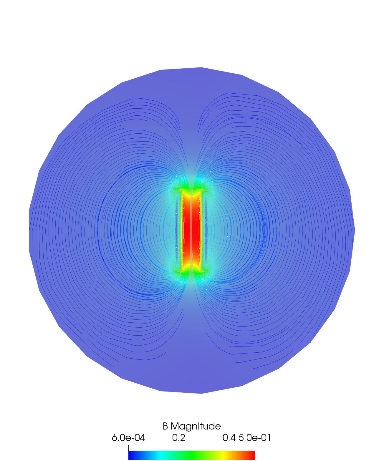 |
3D
load "gmsh"

//Parameters
real Mu0 = 4.*pi*1.e-7; //Vacuum magnetic permeability
real MuC = 1.25e-6; //Copper magnetic permeability
real J0 = 500.e4; //Current density

//Mesh
real R = 2.;
real H = 1.;
real Rint = 0.1;
real Rext = 0.2;

int Coil = 10;
int BoxWall = 1;

mesh3 Th = gmshload3("Magnetostatic3D.msh");

//FESpaces
func Pk = P2;
fespace Ah(Th, [Pk, Pk, Pk]);
Ah [Ax, Ay, Az] = [0, 0, 0];

//Macro
macro Curl(Ax, Ay, Az) [dy(Az)-dz(Ay), dz(Ax)-dx(Az), dx(Ay)-dy(Ax)] //
macro Divergence(Ax, Ay, Az) (dx(Ax) + dy(Ay) + dz(Az)) //

//Current
func r = sqrt(x^2+z^2);
Ah [Jx, Jy, Jz] = J0*[
cos(atan2(z, x)+pi/2.) * (r >= Rint)_(r <= Rext)_(y >= -H/2.)_(y <= H/2.),
0,
sin(atan2(z, x)+pi/2.) _ (r >= Rint)_(r <= Rext)_(y >= -H/2.)\*(y <= H/2.)
];

//Problem
func Mu = Mu0 + (MuC-Mu0)_(region==Coil);
func Nu = 1. / Mu;
varf vLaplacian ([Ax, Ay, Az], [AAx, AAy, AAz])
= int3d(Th)(
Nu _ Curl(Ax, Ay, Az)' _ Curl(AAx, AAy, AAz) + (1./Mu) _ Divergence(Ax, Ay, Az) _ Divergence(AAx, AAy, AAz)
) - int3d(Th)(
[Jx, Jy, Jz]' _ [AAx, AAy, AAz]
) + on(BoxWall, Ax=0, Ay=0, Az=0)
;

matrix<real> Laplacian = vLaplacian(Ah, Ah, solver=sparsesolver);
real[int] LaplacianBoundary = vLaplacian(0, Ah);
Ax[] = Laplacian^-1 \* LaplacianBoundary;

//Magnetic induction
Ah [Bx, By, Bz];
[Bx, By, Bz] = Curl(Ax, Ay, Az);

//Magnetic field
Ah [Hx, Hy, Hz];
[Hx, Hy, Hz] = Nu \* [Bx, By, Bz];| Result - Magnetic induction |
|---|
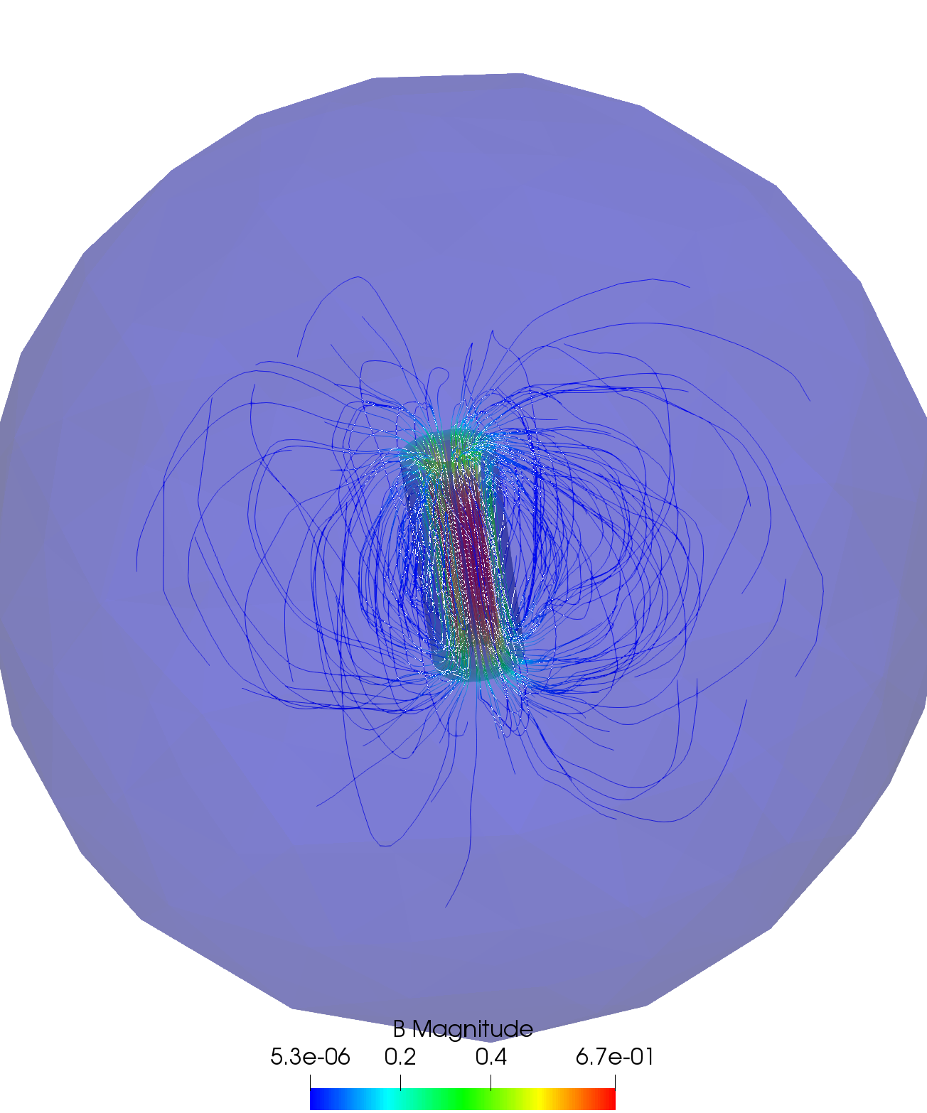 |
Optional
Gmsh script for the 3D mesh:
//////////////////
///Optimization///
//////////////////
Mesh.Optimize = 1;

////////////////
///Parameters/// include in the Gmsh GUI
////////////////
DefineConstant
[
R = {2., Name "Geometry/01 «Infinite» boundary radius"},
LM = {1., Name "Geometry/02 Magnet length"},
RMext = {0.2, Name "Geometry/03 Magnet external radius"},
RMint = {0.1, Name "Geometry/04 Magnet internal radius"},
h = {1., Name "Mesh/01 Characteristic length for boundary"},
hM = {0.05, Name "Mesh/02 Characteristic length for magnet"}
];

//////////////////////
///Global variables///
//////////////////////
Wall[] = {};
MagnetUp[] = {};
MagnetDown[] = {};
MagnetMid[] = {};

///////////////////
///Global sphere///
///////////////////
p = newp;
Point(p+0) = {0, 0, 0, h};
Point(p+1) = {R, 0, 0, h};
Point(p+2) = {0, R, 0, h};
Point(p+3) = {-R, 0, 0, h};
Point(p+4) = {0, -R, 0, h};

l = newl;
Circle(l+0) = {p+1, p+0, p+2};
Circle(l+1) = {p+2, p+0, p+3};
Circle(l+2) = {p+3, p+0, p+4};
Circle(l+3) = {p+4, p+0, p+1};

D1[] = Duplicata {
Line{l+0, l+1, l+2, l+3};
};
//Printf("D1 :", D1[0], D1[1], D1[2], D1[3]);

Rotate { {1, 0, 0}, {0, 0, 0}, Pi/2.} {
Line{D1[0], D1[1], D1[2], D1[3]};
}

D2[] = Duplicata {
Line{l+0, l+1, l+2, l+3};
};
//Printf("D2 :", D2[0], D2[1], D2[2], D2[3]);

Rotate { {0, 1, 0}, {0, 0, 0}, Pi/2.} {
Line{D2[0], D2[1], D2[2], D2[3]};
}

ll =newll;
Line Loop(ll+0) = {l+0, D2[1], -D1[0]};
Line Loop(ll+1) = {l+0, D1[3], -D2[0]};
Line Loop(ll+2) = {l+1, D1[2], D2[0]};
Line Loop(ll+3) = {l+1, -D1[1], -D2[1]};
Line Loop(ll+4) = {l+2, D2[3], -D1[2]};
Line Loop(ll+5) = {l+2, -D2[2], D1[1]};
Line Loop(ll+6) = {l+3, -D1[3], -D2[3]};
Line Loop(ll+7) = {l+3, D1[0], D2[2]};

s = news;
Ruled Surface(s+0) = {ll+0}; Wall[0] = s+0;
Ruled Surface(s+1) = {ll+1}; Wall[1] = s+1;
Ruled Surface(s+2) = {ll+2}; Wall[2] = s+2;
Ruled Surface(s+3) = {ll+3}; Wall[3] = s+3;
Ruled Surface(s+4) = {ll+4}; Wall[4] = s+4;
Ruled Surface(s+5) = {ll+5}; Wall[5] = s+5;
Ruled Surface(s+6) = {ll+6}; Wall[6] = s+6;
Ruled Surface(s+7) = {ll+7}; Wall[7] = s+7;

////////////
///Magnet///
////////////
pext = newp;
Point(pext+0) = {0, 0, -LM/2., hM};
Point(pext+1) = {RMext, 0, -LM/2., hM};
Point(pext+2) = {0, RMext, -LM/2., hM};
Point(pext+3) = {-RMext, 0, -LM/2., hM};
Point(pext+4) = {0, -RMext, -LM/2., hM};

Point(pext+5) = {0, 0, LM/2., hM};
Point(pext+6) = {RMext, 0, LM/2., hM};
Point(pext+7) = {0, RMext, LM/2., hM};
Point(pext+8) = {-RMext, 0, LM/2., hM};
Point(pext+9) = {0, -RMext, LM/2., hM};

lext = newl;
Circle(lext+0) = {pext+1, pext+0, pext+2};
Circle(lext+1) = {pext+2, pext+0, pext+3};
Circle(lext+2) = {pext+3, pext+0, pext+4};
Circle(lext+3) = {pext+4, pext+0, pext+1};

Circle(lext+4) = {pext+6, pext+5, pext+7};
Circle(lext+5) = {pext+7, pext+5, pext+8};
Circle(lext+6) = {pext+8, pext+5, pext+9};
Circle(lext+7) = {pext+9, pext+5, pext+6};

Line(lext+8) = {pext+1, pext+6};
Line(lext+9) = {pext+2, pext+7};
Line(lext+10) = {pext+3, pext+8};
Line(lext+11) = {pext+4, pext+9};

llext = newll;
Line Loop(llext+0) = {lext+0, lext+9, -(lext+4), -(lext+8)};
Line Loop(llext+1) = {lext+1, lext+10 ,-(lext+5), -(lext+9)};
Line Loop(llext+2) = {lext+2, lext+11, -(lext+6), -(lext+10)};
Line Loop(llext+3) = {lext+3, lext+8, -(lext+7), -(lext+11)};

sext = news;
Ruled Surface(sext+0) = {llext+0}; MagnetMid[0] = sext+0;
Ruled Surface(sext+1) = {llext+1}; MagnetMid[1] = sext+1;
Ruled Surface(sext+2) = {llext+2}; MagnetMid[2] = sext+2;
Ruled Surface(sext+3) = {llext+3}; MagnetMid[3] = sext+3;

Rotate { {0, 1, 0}, {0, 0, 0}, Pi/2. } {
Surface{sext+0, sext+1, sext+2, sext+3};
}
Rotate { {0, 0, 1}, {0, 0, 0}, Pi/2. } {
Surface{sext+0, sext+1, sext+2, sext+3};
}

pint = newp;
Point(pint+0) = {0, 0, -LM/2., hM};
Point(pint+1) = {RMint, 0, -LM/2., hM};
Point(pint+2) = {0, RMint, -LM/2., hM};
Point(pint+3) = {-RMint, 0, -LM/2., hM};
Point(pint+4) = {0, -RMint, -LM/2., hM};

Point(pint+5) = {0, 0, LM/2., hM};
Point(pint+6) = {RMint, 0, LM/2., hM};
Point(pint+7) = {0, RMint, LM/2., hM};
Point(pint+8) = {-RMint, 0, LM/2., hM};
Point(pint+9) = {0, -RMint, LM/2., hM};

lint = newl;
Circle(lint+0) = {pint+1, pint+0, pint+2};
Circle(lint+1) = {pint+2, pint+0, pint+3};
Circle(lint+2) = {pint+3, pint+0, pint+4};
Circle(lint+3) = {pint+4, pint+0, pint+1};

Circle(lint+4) = {pint+6, pint+5, pint+7};
Circle(lint+5) = {pint+7, pint+5, pint+8};
Circle(lint+6) = {pint+8, pint+5, pint+9};
Circle(lint+7) = {pint+9, pint+5, pint+6};

Line(lint+8) = {pint+1, pint+6};
Line(lint+9) = {pint+2, pint+7};
Line(lint+10) = {pint+3, pint+8};
Line(lint+11) = {pint+4, pint+9};

llint = newll;
Line Loop(llint+0) = {lint+0, lint+9, -(lint+4), -(lint+8)};
Line Loop(llint+1) = {lint+1, lint+10 ,-(lint+5), -(lint+9)};
Line Loop(llint+2) = {lint+2, lint+11, -(lint+6), -(lint+10)};
Line Loop(llint+3) = {lint+3, lint+8, -(lint+7), -(lint+11)};

sint = news;
Ruled Surface(sint+0) = {llint+0}; MagnetMid[4] = sint+0;
Ruled Surface(sint+1) = {llint+1}; MagnetMid[5] = sint+1;
Ruled Surface(sint+2) = {llint+2}; MagnetMid[6] = sint+2;
Ruled Surface(sint+3) = {llint+3}; MagnetMid[7] = sint+3;

Rotate { {0, 1, 0}, {0, 0, 0}, Pi/2. } {
Surface{sint+0, sint+1, sint+2, sint+3};
}
Rotate { {0, 0, 1}, {0, 0, 0}, Pi/2. } {
Surface{sint+0, sint+1, sint+2, sint+3};
}

l = newl;
Line(l+0) = {pext+1, pint+1};
Line(l+1) = {pext+2, pint+2};
Line(l+2) = {pext+3, pint+3};
Line(l+3) = {pext+4, pint+4};
Line(l+4) = {pext+6, pint+6};
Line(l+5) = {pext+7, pint+7};
Line(l+6) = {pext+8, pint+8};
Line(l+7) = {pext+9, pint+9};

ll = newll;
Line Lopp(ll+0) = {lext+0, l+1, -(lint+0), -(l+0)};
Line Lopp(ll+1) = {lext+1, l+2, -(lint+1), -(l+1)};
Line Lopp(ll+2) = {lext+2, l+3, -(lint+2), -(l+2)};
Line Lopp(ll+3) = {lext+3, l+0, -(lint+3), -(l+3)};

Line Lopp(ll+4) = {lext+4, l+5, -(lint+4), -(l+4)};
Line Lopp(ll+5) = {lext+5, l+6, -(lint+5), -(l+5)};
Line Lopp(ll+6) = {lext+6, l+7, -(lint+6), -(l+6)};
Line Lopp(ll+7) = {lext+7, l+4, -(lint+7), -(l+7)};

s = news;
Ruled Surface(s+0) = {ll+0}; MagnetDown[0] = s+0;
Ruled Surface(s+1) = {ll+1}; MagnetDown[1] = s+1;
Ruled Surface(s+2) = {ll+2}; MagnetDown[2] = s+2;
Ruled Surface(s+3) = {ll+3}; MagnetDown[3] = s+3;

Ruled Surface(s+4) = {ll+4}; MagnetUp[0] = s+4;
Ruled Surface(s+5) = {ll+5}; MagnetUp[1] = s+5;
Ruled Surface(s+6) = {ll+6}; MagnetUp[2] = s+6;
Ruled Surface(s+7) = {ll+7}; MagnetUp[3] = s+7;

///////////////////////
///Physical surfaces///
///////////////////////
WALL = 1;
MAGNETUP = 2;
MAGNETDOWN = 3;
MAGNETMID = 4;

Physical Surface(WALL) = {Wall[]};
Physical Surface(MAGNETUP) = {MagnetUp[]};
Physical Surface(MAGNETDOWN) = {MagnetDown[]};
Physical Surface(MAGNETMID) = {MagnetMid[]};

////////////
///Volume///
////////////
sl = newsl;
Surface Loop(sl+0) = {Wall[]};
Surface Loop(sl+1) = {MagnetDown[], MagnetUp[], MagnetMid[]};

v = newv;
Volume(v+0) = {sl+1};
Volume(v+1) = {sl+0, (sl+1)};

//////////////////////
///Physical volumes///
//////////////////////
MAGNETVOLUME = 10;
VACUUMVOLUME = 20;

Physical Volume(MAGNETVOLUME) = {v+0};
Physical Volume(VACUUMVOLUME) = {v+1};| Mesh |
|---|
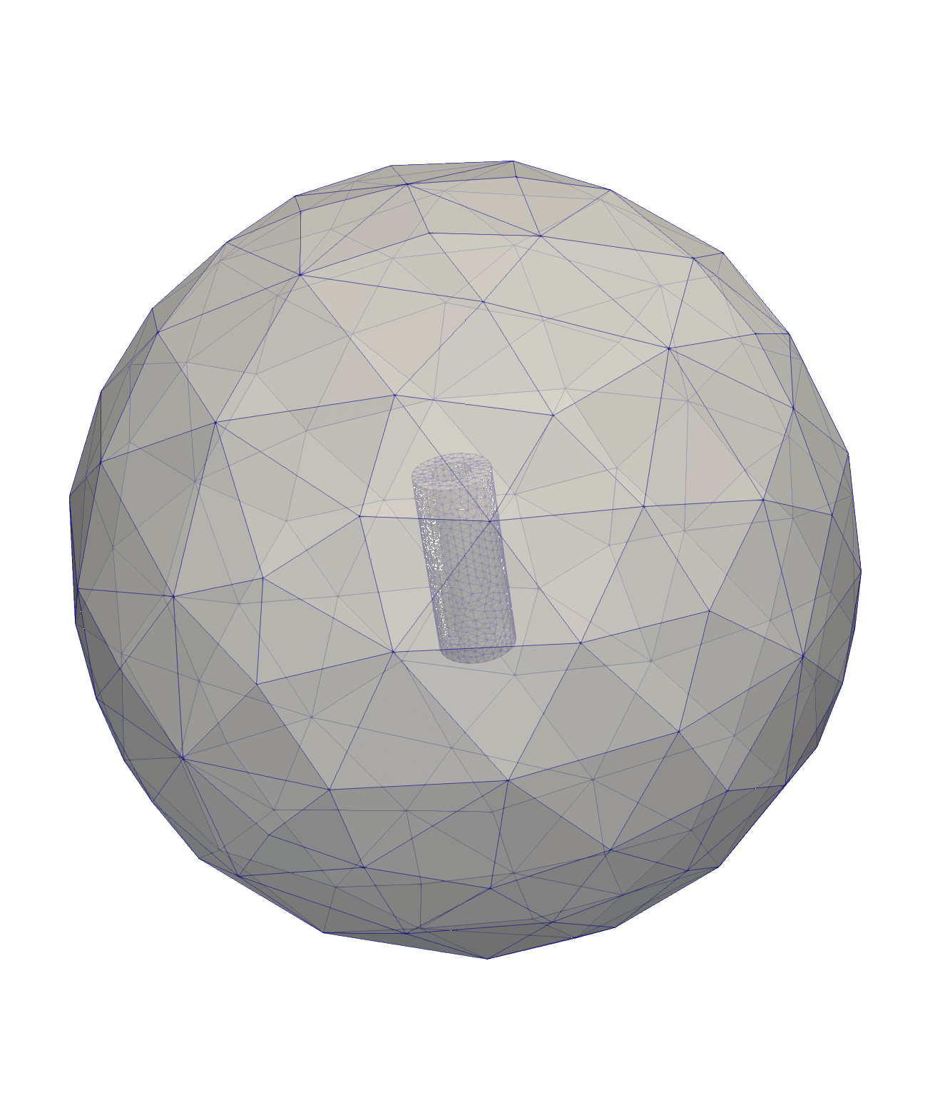 |
Validation
Taking the Biot and Savart formula, P a point on the solenoid , M a point in the space, $\overrightarrow{dl}$ the direction of the current at point P. $ \displaystyle{\overrightarrow{Jfil}=Jfil * \overrightarrow{PM}} $
$ \displaystyle{ {As : }dPM = \overrightarrow{PM} / |PM| = \overrightarrow{PM} / \sqrt{\overrightarrow{PM}^2} = \overrightarrow{PM} / \sqrt{( \overrightarrow{PM} * \overrightarrow{PM} )} }$
$
\displaystyle{
\overrightarrow{dB} = Jfil * u0/(4 * \pi) * \frac{ \overrightarrow{dl} \wedge \overrightarrow{dPM}} {PM^2} = \frac{Jfil * u0}{4 * \pi} * \begin{pmatrix} dl1 \cr dl2 \cr dl3 \end{pmatrix} \wedge \frac{ \begin{pmatrix} x_M - x_P \cr y_M - y_P \cr z_M - z_P \end{pmatrix} } { ( (x_M - x_P)^2 + (y_M - y_P)^2 + (z_M - z_P)^2 )^{3/2} }
}$
$
\displaystyle{
P\colon
\begin{pmatrix}
R * cos(\theta) \cr
ycerc \cr
R * sin(\theta)
\end{pmatrix}
{ , }
M\colon
\begin{pmatrix}
0 \cr
ya \cr
0
\end{pmatrix}
{ , }
\overrightarrow{dl}
\colon
\begin{pmatrix}
sin(\theta) \cr
0 \cr
-cos(\theta)
\end{pmatrix}
{ , }
\overrightarrow{PM}
\colon
\begin{pmatrix}
-R * cos(\theta) \cr
ya-ycerc \cr
-R * sin(\theta)
\end{pmatrix}
\implies
{ dB= }
\begin{pmatrix}
\frac{ Jfil * cos(\theta) * u0 * (ya-ycerc) } { 4 * \pi * ((ya-ycerc)^2+R^2)^{3/2} } \cr
\frac{ Jfil * R * u0 } { 4 * \pi * ((ya-ycerc)^2+R^2)^{3/2} } \cr
\frac{ Jfil * sin(\theta) * u0 * (ya-ycerc) } { 4 * \pi * ((ya-ycerc)^2+R^2)^{3/2} }
\end{pmatrix}
}$
We are only interested in By according to the $\overrightarrow{y}$ axis. Because of the cylindrical coordinates, we have to multiply the term dBy by R. We integrate on $\theta$ angle view of the coil, including the height of the coil ycerc and R radius of the coil.
$
\displaystyle{
By = \int_{0}^{2 * \pi}\int_{R1}^{R2}\int_{-MagnetHeight/2}^{MagnetHeight/2} R * \frac{ Jfil * R * u0 } { 4 * \pi * ((ya-ycerc)^2+R^2)^{(3/2)} } * d\theta * dr * dy = \int R * (Jfil * R * u0/2) * }$
$
\displaystyle{\left( \frac{2 * ya+MagnetHeight} {R^2 * \sqrt{4 * ya^2+4 * MagnetHeight * ya+MagnetHeight^2+4 * R^2} } - \frac{ 2 * ya-MagnetHeight } {R^2 * \sqrt{4 * ya^2-4 * MagnetHeight * ya+MagnetHeight^2+4 * R^2} } \right) * dr
}$
$
\displaystyle{
By= Jfil * u0 * /4 * \left [ (2 * ya+MagnetHeight) * asinh (\frac{2 * R2}{\sqrt{4 * ya^2+4 * MagnetHeight * ya+MagnetHeight^2} })
+(-2 * ya-MagnetHeight) * asinh(\frac{2 * R1}{\sqrt{4 * ya^2+4 * MagnetHeight * ya+MagnetHeight^2} }) +(MagnetHeight-2 * ya) * asinh(\frac{2 * R2}{\sqrt{4 * ya^2-4 * MagnetHeight * ya+MagnetHeight^2} }) +(2 * ya-MagnetHeight) * asinh(\frac{2 * R1}{\sqrt{4 * ya^2-4 * MagnetHeight * ya+MagnetHeight^2} }) \right ]
}$
At the center, z=0,y=0,
$
\displaystyle{By (0,0,0) = Jfil * u0 * MagnetHeight/2 * ( \operatorname{asinh}( \frac{2 * R2}{MagnetHeight}) -\operatorname{asinh}( \frac{2 * R1}{MagnetHeight}) ) }$
The function asinh , inverse hyperbolic sinus , is unavailable under Paraview. Also the square function become 0 at the point $y= \pm MagnetHeight/2$, the ends of the solenoid . We need to develop again using the following rules.
$ \displaystyle{ \operatorname{asinh(x)} = log( x + \sqrt{x^2+1} ) { et } asinh(a/b) = log( a/b + \sqrt{(a/b)^2+1} ) = log (a+ \sqrt{a^2+b^2})-log(b); }$
$ \displaystyle{By (0,ya,0) = Jfil * u0/4 * ( (2 * ya+MagnetHeight) * (\log( \sqrt{(2 * ya+MagnetHeight)^2+4 * R2^2}+2 * R2 ) - \log( \sqrt{(2 * ya+MagnetHeight)^2+4 * R1^2}+2 * R1 ) ) +(2 * ya-MagnetHeight) * ( \log( \sqrt{(2 * ya-MagnetHeight)^2+4 * R1^2}+2 * R1 ) - \log( \sqrt{(2 * ya-MagnetHeight)^2+4 * R2^2}+2 * R2 ) ) ) }$
In the code , add the lines to compute the formula and produce a cut.
Ah Byanaly;

Byanaly  =    -(J0*Mu0*((2*y+MagnetHeight)*(log(sqrt((2*y+MagnetHeight)^2+4*MagnetExternalRadius^2)+2*MagnetExternalRadius)-log(sqrt((2*y+MagnetHeight)^2+4*MagnetInternalRadius^2)+2*MagnetInternalRadius))-(2*y-MagnetHeight)*(log(sqrt((2*y-MagnetHeight)^2+4*MagnetExternalRadius^2)+2*MagnetExternalRadius)-log(sqrt((2*y-MagnetHeight)^2+4*MagnetInternalRadius^2)+2*MagnetInternalRadius))))/4   ;


// Compute a cut
int n = 100;
real[int] xx(n), yy(n) ,  yy2(n);
for (int i =  0; i < n; i++){
y = i/real(n)*BoxRadius*2.0 -BoxRadius;
x = 0.0;
xx[i] = i;
yy[i] = By; // Value of uh at point (i/10., i/10.)
yy2[i] = Byanaly;
}

plot([xx, yy], [xx, yy2] , wait=true);
An another way is the Gauss-Legendre quadrature. For an easy geometry, it can integrate and give the field anywhere in the space except in the conductor of solenoid.
See the link: lien wikipedia FR
To resume, an integral of f(x) become a sum of the function f(x) at xn specific points (roots of a Legendre polynome xn), weighted by an. $ \displaystyle{Y=\int f(x) = \sum_i^n an_i * f(x_i^n)} $
With the same parameters , except M in the plan (x,y,0) so M has the coordinates (xa,ya,0), giving:
$\displaystyle{
{ dB= Jfil * u0 }/4/\pi *
\begin{pmatrix}
\frac{ cos(\theta) * (ya-ycerc) } { ( (ya-ycerc)^2+(xa-R * cos(\theta))^2+R^2 * sin(\theta)^2)^{(3/2)} }
\frac{ (R * sin(\theta)^2-cos(\theta) * (xa-R * cos(\theta) ) ) } { ((ya-ycerc)^2+(xa-R * cos(\theta))^2+R^2 * sin(\theta)^2)^{(3/2)} }
\frac{ sin(\theta) * (ya-ycerc) } { ((ya-ycerc)^2+(xa-R * cos(\theta))^2+R^2 * sin(\theta)^2)^{(3/2)} }
\end{pmatrix}
}$
To avoid an triple integration, we “pre-integrate” along the axis of the solenoid and let two integrals along $\theta$ and R. The “pre-integration” is named f(x) for convenience. An term R is added due to the cylindricals coordinates.
$ \displaystyle{ By = \iint_{\theta=0,\ R=R1}^{\theta=2\pi,\ R=R2} f(\theta,R) * d\theta * dr = \iint -R * Jfil * u0/4/\pi * (cos(\theta) * xa-R) * \left( \frac { ((2 * ya+MagnetHeight) * \sqrt{(4 * ya^2+4 * MagnetHeight * ya+4 * xa^2-8 * R * cos(\theta) * xa+MagnetHeight^2+4 * R^2)} )} { ((4 * xa^2-8 * R * cos(\theta) * xa+4 * R^2) * ya^2+(4 * MagnetHeight * xa^2-8 * R * MagnetHeight * cos(\theta) * xa+4 * R^2 * MagnetHeight) * ya +4 * xa^4-16 * R * cos(\theta) * xa^3+(16 * R^2 * cos(\theta)^2+MagnetHeight^2+8 * R^2) * xa^2+(-2 * R * MagnetHeight^2-16 * R^3) * cos(\theta) * xa+R^2 * MagnetHeight^2+4 * R^4) } - \frac { -((2 * ya-MagnetHeight) * \sqrt{(4 * ya^2-4 * MagnetHeight * ya+4 * xa^2-8 * R * cos(\theta) * xa+MagnetHeight^2+4 * R^2)}) } { ((4 * xa^2-8 * R * cos(\theta) * xa+4 * R^2) * ya^2+(-4 * MagnetHeight * xa^2+8 * R * MagnetHeight * cos(\theta) * xa-4 * R^2 * MagnetHeight) * ya +4 * xa^4-16 * R * cos(\theta) * xa^3+(16 * R^2 * cos(\theta)^2+MagnetHeight^2+8 * R^2) * xa^2+(-2 * R * MagnetHeight^2-16 * R^3) * cos(\theta) * xa+R^2 * MagnetHeight^2+4 * R^4) } \right) * d\theta * dr }$
The integration is better with an higher degree of the polynomials used, n is the quadrature degree , an_i and an_j are the weights for the integral along $\theta$ and R. $\theta_i$ and $R_i$ are the discrete values for $\theta$ et R. Legendre polynomials is valid on [-1;1], change the domain is necessary for $\theta$ and R respectively $[0;\pi]$ et [R1;R2].
$ \displaystyle{ \theta \in [0;\pi] \implies \theta_i^n = (2 * \pi -0)/2.0 * x_i + (2 * \pi +0) /2 { } R \in [R1;R2] \implies R_i^n = (MagnetExternalRadius - MagnetInternalRadius)/2.0 * x_j + (MagnetExternalRadius + MagnetInternalRadius)/2.0 }$
$ \displaystyle{ By \simeq \sum_i^n \sum_j^n an_i * an_j * (\theta_{max}-\theta_{min})/2 * (Rbobine_{max} - Rbobine_{min})/2 * f(\theta_i,R_j) = \sum_i^n \sum_j^n an_i * an_j * (2\pi -0)/2.0 *(MagnetExternalRadius - MagnetInternalRadius)/2.0 * f(\theta_i,R_j) }$
The computing take 3/4 h with an laptop. Looking the curves on Paraview, the results by quadrature method is very close to the analytical formulation. The intensity of By is tighter than the FEM results.
The code :
/*

Calcul du champ par méthode de Gauss Legendre

*/

load iovtk

Ah Bymet;

int degpoly= 9;
real[int]  xn= [    0.000000000000000, 0.324253423403809,  0.613371432700590, 0.836031107326636, 0.968160239507626, -0.324253423403809, -0.613371432700590, -0.836031107326636, -0.968160239507626   ];
real[int]  an=[  0.330239355001260,0.312347077040003,0.260610696402935,0.180648160694857,0.081274388361574,0.312347077040003,0.260610696402935,0.180648160694857,0.081274388361574  ];


real rayonc = 0.0;
real theta2 = 0.0;
real ycerc = 0.0;


for (int j =  0; j < degpoly; j++){
for (int i =  0; i < degpoly; i++){


theta2 =   (2*pi -0)/2.0 *xn[i]  +  (2*pi +0) /2 ;
rayonc  =   (MagnetExternalRadius - MagnetInternalRadius)/2.0 * xn[j] + (MagnetExternalRadius + MagnetInternalRadius)/2.0 ;


cout << "iteration i = "<< i << "  iteration j = "<< j  << endl;


Bymet =  Bymet +     an[i]*an[j]* (2*pi -0)/2.0 *(MagnetExternalRadius - MagnetInternalRadius)/2.0 * rayonc * (J0*Mu0*(rayonc*cos(theta2)^2-sin(theta2)*(x-rayonc*sin(theta2)))*(((2*y+MagnetHeight)*sqrt(4*y^2+4*MagnetHeight*y+4*x^2-8*rayonc*sin(theta2)*x+4*rayonc^2*sin(theta2)^2+4*rayonc^2*cos(theta2)^2+MagnetHeight^2))/((4*x^2-8*rayonc*sin(theta2)*x+4*rayonc^2*sin(theta2)^2+4*rayonc^2*cos(theta2)^2)*y^2+(4*MagnetHeight*x^2-8*MagnetHeight*rayonc*sin(theta2)*x+4*MagnetHeight*rayonc^2*sin(theta2)^2+4*MagnetHeight*rayonc^2*cos(theta2)^2)*y+4*x^4-16*rayonc*sin(theta2)*x^3+(24*rayonc^2*sin(theta2)^2+8*rayonc^2*cos(theta2)^2+MagnetHeight^2)*x^2+(((-16*rayonc^3*cos(theta2)^2)-2*MagnetHeight^2*rayonc)*sin(theta2)-16*rayonc^3*sin(theta2)^3)*x+4*rayonc^4*sin(theta2)^4+(8*rayonc^4*cos(theta2)^2+MagnetHeight^2*rayonc^2)*sin(theta2)^2+4*rayonc^4*cos(theta2)^4+MagnetHeight^2*rayonc^2*cos(theta2)^2)-((2*y-MagnetHeight)*sqrt(4*y^2-4*MagnetHeight*y+4*x^2-8*rayonc*sin(theta2)*x+4*rayonc^2*sin(theta2)^2+4*rayonc^2*cos(theta2)^2+MagnetHeight^2))/((4*x^2-8*rayonc*sin(theta2)*x+4*rayonc^2*sin(theta2)^2+4*rayonc^2*cos(theta2)^2)*y^2+((-4*MagnetHeight*x^2)+8*MagnetHeight*rayonc*sin(theta2)*x-4*MagnetHeight*rayonc^2*sin(theta2)^2-4*MagnetHeight*rayonc^2*cos(theta2)^2)*y+4*x^4-16*rayonc*sin(theta2)*x^3+(24*rayonc^2*sin(theta2)^2+8*rayonc^2*cos(theta2)^2+MagnetHeight^2)*x^2+(((-16*rayonc^3*cos(theta2)^2)-2*MagnetHeight^2*rayonc)*sin(theta2)-16*rayonc^3*sin(theta2)^3)*x+4*rayonc^4*sin(theta2)^4+(8*rayonc^4*cos(theta2)^2+MagnetHeight^2*rayonc^2)*sin(theta2)^2+4*rayonc^4*cos(theta2)^4+MagnetHeight^2*rayonc^2*cos(theta2)^2)))/(4*pi);


}
//cout << "iteration k = "<< k << "  iteration j = "<< j  << endl;
//cout << "iteration i = "<< i << "  iteration j = "<< j  << endl;

}

savevtk("/home/users/Documents/sortiemethodGL.vtk",Th, Bymet , dataname="B", bin=false );
Authors
Author: Simon Garnotel Author: tess35 for validation part