
Signorini’s contact problem with Interior point optimizer (IPOPT)
Algorithm to solve the contact between an elastic body and a rigid foundation (obstacle).
Problem
We consider Signorini’s problem which is the contact between a body and a rigid foundation. We treat only the linear elastic materials case and the plane strain hypothesis (2D) is assumed. Let $\Omega \subset \mathbb{R}^{2}$ denotes the body and $\Gamma= \partial \Omega$ its boundary. $\Gamma_{0} \subset \Gamma$ denotes the boundary part where a displacement is imposed, $\Gamma_{1} \subset \Gamma$ is the boundary part where a traction vector $\mathbf{t}$ is applied, finally $\Gamma_{C} \subset \Gamma$ denotes the potential contact area.
By imposing a null displacement on $\Gamma_{0}$, the displacement admissible set is defined as follows
$ \displaystyle{ \mathbf{V}= \left\lbrace \mathbf{v} \in \left( H^{1}(\Omega)\right)^{2} \, | \, \mathbf{v}=0 \text{ on } \Gamma_{0} \right\rbrace } $
The total potential energy $E_{p}$ is given by the following
$ \displaystyle{ E_{p}(\mathbf{v})= \frac{1}{2} \int_{\Omega} \boldsymbol{\sigma}^{T}.\boldsymbol{\epsilon} \, dV - \int_{\Gamma_{1}} \mathbf{t} . \mathbf{v} \, dA } $
where $\boldsymbol{\epsilon}$ and $\boldsymbol{\sigma}$ is respectively the strain vector and the stress vector, if $\mathbf{v}=(v_{1},v_{2})$ we have
$ \displaystyle{ \boldsymbol{\epsilon}=\begin{pmatrix} \epsilon_{x} \newline \epsilon_{y} \newline \gamma_{xy} \end{pmatrix}=\begin{pmatrix} \frac{\partial v_{1}}{\partial x} \newline \frac{\partial v_{2}}{\partial y} \newline \frac{\partial v_{1}}{\partial y} + \frac{\partial v_{2}}{\partial x} \end{pmatrix} \, \, \, and \, \, \, \boldsymbol{\sigma} = \mathbf{D} \boldsymbol{\epsilon} } $
In addition
$ \displaystyle{ \mathbf{D}=\frac{E}{(1+\nu)(1-2\nu)} \, \begin{bmatrix} 1-\nu & \nu & 0 \newline \nu & 1-\nu & 0 \newline 0 & 0 & \frac{1-2\nu}{2} \end{bmatrix} } $
with $E$ the Young’s modulus and $\nu$ the Poisson’s ratio.
The solution (the displacement field) of the contact problem involving a linear elastic body, can be written as the following minimization problem
$ \displaystyle{ \mathbf{u}= \underset{\mathbf{v} \in \mathbf{K}}{\text{argmin}} \, (E_{p}(\mathbf{v})) } $
where $\mathbf{K}$ is the set describing the non-penetration condition for the Signorini’s problem, and is given by
$ \displaystyle{ \mathbf{K} = \left\lbrace \mathbf{v} \in \mathbf{V} \, | \, (\mathbf{v}+\mathbf{X}-\bar{\mathbf{X}}).\mathbf{n} \geq 0 \text{ on } \Gamma_{C} \right\rbrace } $
where $\mathbf{X}$ is the position in the initial configuration, $\bar{\mathbf{X}}$ its projection on the obstacle and $\mathbf{n}$ is the outward unit normal vector at $\bar{\mathbf{X}}$.
Discretization
In order to describe the non-pentration between the body $\Omega$ and the obstacle, the node-to-segment discretization is used, in other words the body nodes can not penetrate the obstacle. Let $i$ be a node of the body, belonging to the potential contact area $\Gamma_{C}$, then the non-penetration conditions in this case can be given as follows
$ \displaystyle{ (\mathbf{x}^{i}-\bar{\mathbf{x}}^{i}) . \mathbf{n}^{i} \geq 0 \, \, \, \forall \, i=1,\ldots,n_{C} } $
where $n_{C}$ is the number of the contact nodes, $ \mathbf{x}^{i} $ the actual position of the node $i$, $\bar{\mathbf{x}}^{i}$ the projection on the obstacle of $\mathbf{x}^{i}$ which is equal to $\bar{\mathbf{X}}^{i}$, the projection of the initial position, in the case of small displacements. Finally $\mathbf{n}^{i}$ is the outward unit normal vector at $\bar{\mathbf{x}}^{i}$.
In general, better and robust results can be obtained using the weak contact formulation (see [1,2]).
In the case of small deformations, the total potential energy $E_{p}$ can be given as follows
$ \displaystyle{ E_{p}(U)=\frac{1}{2}U^{T}KU - FU } $
where $K$ is the rigidity matrix, $F$ the nodale forces and $U \in \mathbb{R}^{n}$ the displacement field degrees of freedom vector. In addition the non-penetration constraints are linear and can be expressed as follows
$ \displaystyle{ AU + b \geq 0 } $
Finally, the contact problem for the linear elastic body, can be written as the following minimization problem
$ \begin{cases} \underset{V \in \mathbb{R}^{n}}{\text{min}} \, \frac{1}{2}V^{T}KV - FV \newline AV + b \geq 0 \end{cases} $
NB : One can find in [3] another formulation for the Signorini’s problem.
Algorithms
we consider the contact between an elastic arch and a rigid one, due to an applied pressure. A new FreeFEM function, called projection, is used in order to compute the projection points.
Please cite [1] or [2] if you want to use the following code.
Geometry
File Geometry.idp
// Body geometry

// Mesh quality
int nu1  =100;           // Mesh quality for the body
int nu2  =102;           // Mesh quality for the obstacle

// Type of the Finite element space
func Pk1 = P1;	// Finite element space
func Pk2 = P1;	// Finite element space

// Pressure amplitude
real pres=30;

// Amplification
real amplify =1;

// The body
int Contact1  = 1;
int Force1    = 2;
int Symmy     = 3;

real R1=40;
real e1=10;
real R2=R1-e1;
border b11(t=0,pi){x=R1*cos(t);y=R1*sin(t);label=Contact1;}
border b12(t=0,e1){x=-R1+t;y=0.;label=Symmy;}
border b13(t=pi,0){x=R2*cos(t);y=R2*sin(t);label=Force1;}
border b14(t=0,e1){x=R2+t;y=0;label=Symmy;}
mesh Th1=buildmesh(b11(nu1)+b12(nu1/10)+b13(nu1)+b14(nu1/10));

// The obstacle
int Found2    = 4;
int Contact2  = 5;
// Foundation mesh
real R5=50;
real R6=R1+1.;
real e2=R5-R6;
border b21(t=0,pi){x=R5*cos(t);y=R5*sin(t);label=Found2;}
border b22(t=0,e2){x=-R5+t;y=0.;label=Found2;}
border b23(t=pi,0){x=R6*cos(t);y=R6*sin(t);label=Contact2;}
border b24(t=0,e2){x=R6+t;y=0;label=Found2;}
mesh Th2=buildmesh(b21(nu2)+b22(nu2/10)+b23(nu2)+b24(nu2/10));

// The finite element spaces
fespace Wh1(Th1,[Pk1,Pk1]); //FE for the body
fespace Wh2(Th2,[Pk2,Pk2]); //FE for the obstacle (to define the normal vector)
Material parameters
Definition of the elasticity law in 2D.
File Elastic_lin_2d.idp
// Material law

// Density energy for the elastic body and it differentials
real E1=1*1e3; // Young modulus (Pa)
real pois1=0.; // Poisson modulus
real lambda1 = E1*pois1/((1.+pois1)*(1.-2.*pois1)); // Lamé coefficients
real mu1 = E1/(2.*(1.+pois1)) ; // Lamé coefficients
real twomul1=2*mu1+lambda1;
//Elasticity matrix
func AA1 = [[twomul1,lambda1, 0. ], [lambda1,twomul1, 0. ],[ 0. , 0. , mu1 ]];
// Strain vector
macro epsV1(d) ([dx(d[0]),dy(d[1]),dy(d[0])+dx(d[1])]) //
// Strain first differential
macro deps1(d,dd) ([dx((dd)[0]),dy((dd)[1]),dy((dd)[0])+dx((dd)[1])] ) //
//Density energy for elastic bodies
macro W2d1(d)  ((1./2.)*( epsV1(d)'* AA1 *epsV1(d))) //
// Density energy first differential
macro dW2d1(d,dd)(
(1./2.)*( epsV1(d)'*AA1*deps1(d,dd)) + (1./2.)*((deps1(d,dd))'*AA1*epsV1(d))
) //
// Density energy second differential
macro ddW2d1(d,dd,ddd)(
(1./2.)*( deps1(d,ddd)'*AA1*deps1(d,dd)) + (1./2.)*((deps1(d,dd))'*AA1*deps1(d,ddd))
) //

macro Sigma1(d) ( AA1*epsV1(d) ) // The stress vector
Minimization algorithm
// Linear elasticity is assumed
// The contact conditions are described by the node-to-segment discretization (each node can not penetrate the obstacle)
load "ff-Ipopt" // Load the interior point optimizer
load "msh3" // Even if we are in 2D case, it's used to compute the projection points
include "Elastic_lin_2d.idp" // Material data
include "Geometry.idp" // Geometrical data
//Degree of Freedom
int ndof1=Wh1.ndof; // Number of the degree of freedom for the body
meshL Lh = extract(Th2); // The border of Th2 (used to compute the projection points)
// Define the normal field
varf normvar([Dx, Dy], [v1, v2]) = int1d(Th2,Contact2)(v1*N.x+v2*N.y);
real[int] normfieldvec = normvar(0, Wh2, tgv=1); // Not normalized
Wh2 [normx,normy];
normx[]=normfieldvec;
// Vectors & arrays for Contact
int[int] Jb1;
real[int] Xb1(0);
int nC1=0;
//
// Extract contact borders for the body
varf vborder1([Dx, Dy], [v1, v2]) = on(Contact1, Dx=1, Dy=1);
real[int] onBorder1 = vborder1(0, Wh1, tgv=1);
int numB1 = onBorder1.sum;
Jb1.resize(numB1);
int k = 0;
for [i, B1i:onBorder1]
if (B1i) { Jb1[k] = i; k++; }
// End extract borders for the body
// Working space (All internal variables are deleted after)
{
Wh1 [xx1,yy1]=[x,y]; // position vector
nC1=Jb1.n/2; // Constraints number
Xb1.resize(2*nC1);
Xb1=xx1[](Jb1); // Coord on Border x, y
} // End working space
Wh1 [U1x, U1y]; // Displacement for the body
///////////////////////////////////////////////////////////
matrix KRIG;
// Compute rigidity matrix (Linear elasticity)
Wh1 [D01x, D01y];
D01x[] = 0.;
varf ddW1 ([Dx, Dy], [Vx, Vy])
= int2d(Th1)(ddW2d1([D01x, D01y], [Dx, Dy], [Vx, Vy]));
KRIG = ddW1(Wh1, Wh1); // Rigidity matrix for the body
// Compute external forces
varf dW1 ([Dx, Dy], [Vx, Vy]) = int1d(Th1,Force1)(-Vx*pres*N.x-Vy*pres*N.y);
real[int] FEXT = dW1(0, Wh1); // External forces for the body
///////////////////////////////////////////////////////////
real[int] DIS(ndof1); // The Unknown displacement of the body
DIS=0.; // Initial displacement
real cpu0=clock(); // Time before resolution
real[int] Proj(2*nC1); // (x,y) of the projected points
real[int] norm(2*nC1); // The normal (nx,ny) of the projected points
// Compute the projection points
for(int i=0;i<nC1;i++){
x=Xb1[2*i]; // The abssica of the contact node
y=Xb1[2*i+1]; // The ordinate of the contact node
z=0; // 2D case
int nu; // The border segment number (not used here)
R3 ph;
R3 proj=projection(Lh,nu=nu,Phat=ph); // Projection of the contact node
Proj[2*i] =proj.x; // Abssica of the projection of the contact node
Proj[2*i+1]=proj.y; // Ordinate of the projection of the contact node
norm[2*i]=normx(Proj[2*i],Proj[2*i+1])/( (normx(Proj[2*i],Proj[2*i+1]))^2 + (normy(Proj[2*i],Proj[2*i+1]))^2)^0.5; // The normal x vector at a node
norm[2*i+1]=normy(Proj[2*i],Proj[2*i+1])/( (normx(Proj[2*i],Proj[2*i+1]))^2 + (normy(Proj[2*i],Proj[2*i+1]))^2)^0.5; // The normal y vector at a node
}
//*****ENERGY AND ITS DIFFERENTALS*****
// The Energy of the body
func real iW (real[int] &X) {
real[int] idWW(ndof1);
idWW=KRIG*X;
real res =X'*idWW;
res=0.5*res-X'*FEXT; // Energy = 1/2* (X^T)*K*X - (X^T)*Fext
return res;
}
// End Energy function
// Energy Gradient
func real[int] idW (real[int] &X) {
real[int] idWW(ndof1);
idWW=KRIG*X;
idWW=idWW - FEXT;
return idWW; // The gradient of the total energy
}
// End of the gradient energy
// The Energy Hessian
func matrix iddW (real[int] &X) {
return KRIG;
}
// End of the Hessian energy
//*****CONSTRAINTS AND ITS DIFFERENTALS*****
real[int] Wb1(2*nC1);
//Constraints function
func real[int] Cnst2 (real[int] &X) {
real[int] Co(nC1);
Wb1=Xb1;
Wb1 += X(Jb1);
for (int i=0;i<nC1;i++){ // Defining the nC1 constraints (each node is not allowed to penetrate the foundation)
real xpr=Proj[2*i]; // x of the projected point
real ypr=Proj[2*i+1]; // y of the projected point
Co[i]=(Wb1[2*i]-xpr)*norm[2*i]+(Wb1[2*i+1]-ypr)*norm[2*i+1]; // (x-\bar{x}).n >=0
}
return Co;
} //Constraints
// Jacobian of the constraints
real[int,int] Jac1(nC1,ndof1);
matrix JACOB;
JACOB.resize(nC1,ndof1);
{ // The Jacobian of the constraints is constant
for (int i=0;i<nC1;i++){ // Defining the nC1 constraints (each node is not allowed to penetrate the foundation)
JACOB(i,Jb1[2*i])=norm[2*i];
JACOB(i,Jb1[2*i+1])=norm[2*i+1];
}
}
real[int] GAP(nC1);
real[int] NULDIS(ndof1);
NULDIS=0.;
GAP=Cnst2(NULDIS); // Initial Gap
//Constraints (or one can use the constraints function Cnst2 )
func real[int] Cnst (real[int] &X) { //
real[int] AX(nC1);
AX=JACOB*X;
AX+=GAP;
return AX;
} //Constraints
func matrix jacCnst (real[int] &X){
return JACOB;
}
// Hessian of the constraints
matrix Hessian;
func matrix hessianCnst (real[int] &X, real sigma, real[int] &lambda){
Hessian = sigma*iddW(X);
return Hessian;
}
real[int] cl(nC1); cl=0.; // Constraints lower bounds (no upper bounds)
// Boundary conditions for the body
Wh1 [ub11, ub12] = [1e19, 1e19]; // Unbounded in interior
Wh1 [lb11, lb12] = [-1e19, -1e19]; // Unbounded in interior
varf vGamma1([Dx, Dy], [v1, v2]) = on(Symmy, Dx=1, Dy=1); // For Boundary conditions
real[int] onGamma1 = vGamma1(0, Wh1, tgv=1);
Wh1 [ubb11, ubb12] = [ub11,0.]; // Symmetry w.r.t y
Wh1 [lbb11, lbb12] = [lb11,0.]; // Symmetry w.r.t y
ub11[]= onGamma1 ? ubb11[] : ub11[]; // enforcing the boundary condition
lb11[]= onGamma1 ? lbb11[] : lb11[]; // enforcing the boundary condition
IPOPT(iW, idW, hessianCnst, Cnst, jacCnst, DIS, lb=lb11[], ub=ub11[], clb=cl); // Minimize with IPOPT
// Plotting
U1x[]=DIS;
plot(Th1,Th2);
plot(Th1,[U1x, U1y],Th2);
mesh Thm1 = movemesh(Th1, [x+U1x*amplify, y+U1y*amplify]);
plot(Thm1,Th2);
//Compute the stresses
fespace Vh1(Th1,P0);
Vh1 Sigmavm1, sigy1, sigx1, sigxy1, sigz1, sigmar1;
sigx1=Sigma1([U1x, U1y])[0]; // Stress Component
sigy1=Sigma1([U1x, U1y])[1]; // Stress Component
sigxy1=Sigma1([U1x, U1y])[2]; // Stress Component
sigz1=pois1*(sigx1+sigy1); // Stress Component
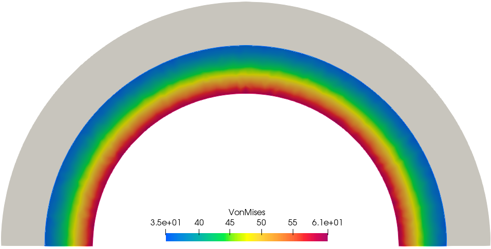
Sigmavm1 =sqrt(0.5*((sigx1-sigy1)^2 + (sigy1-sigz1)^2 + (sigz1-sigx1)^2 )+3*sigxy1^2); // Von-Mises stress
sigmar1=sigx1*(x*x/(x^2+y^2))+sigy1*(y*y/(x^2+y^2)) +2.*sigxy1*(x*y/(x^2+y^2)); // Radial stress
//PLOT
plot(Sigmavm1,value=1,fill=1,cmm="Von Mises");
plot(sigmar1,value=1,fill=1,cmm="Radial stress");
{
load "iovtk"
fespace PVh1(Th1, P0);
PVh1 DDx1=U1x, DDy1=U1y;
PVh1 vm1=Sigmavm1;
int[int] order = [1,1];
string dataname1 = "u VonMises";
savevtk("Signorini_NTS.vtu",Th1,[DDx1, DDy1, 0],vm1,dataname=dataname1, order=order);
savevtk("The_obstacle.vtu",Th2);
}
real cpu1=clock(); // IPOPT resolution time
cout << "------------------------------" << endl;
cout << "RESOLUTION TIME= " << cpu1-cpu0 << endl;
cout << "------------------------------" << endl;| Result - Von Mises stress |
|---|
 |
References
[1] Finite element modeling of mechanical contact problems for industrial applications, H. Houssein, PhD thesis, Sorbonne Université
[2] A symmetric algorithm for solving mechanical contact problems using FreeFEM, H. Houssein, S. Garnotel, F. Hecht (To appear in Computational Methods in Applied Sciences, Springer)
[3] Frictionless contact problem for hyperelastic materials with interior point optimizer, H. Houssein, S. Garnotel, F. Hecht (HAL)
Authors
Author: Houssam Houssein