
Navier-Stokes
Algorithm for solving the 2D and 3D time-dependant Navier-Stokes equations using the characteritics method
Problem
Solve:
\[\left\{ \begin{align*} \rho\frac{\partial\mathbf{u}}{\partial t} + \rho(\mathbf{u}\cdot\nabla\mathbf{u})-\Delta\mathbf{u} + \nabla p &= 0\\ \nabla\cdot\mathbf{u} &= 0 \end{align*} \right.\]Weak form
\[\rho\frac{\partial\mathbf{u}}{\partial t}\mathbf{v} + \rho(\mathbf{u}\cdot\nabla\mathbf{u})\mathbf{v} - \mu\int_{\Omega}{\nabla\mathbf{u}:\nabla\mathbf{v} - p\nabla\cdot\mathbf{v}} - \int_{\partial\Omega}{\left(\nu\frac{\partial\mathbf{u}}{\partial\mathbf{n}}-p\mathbf{n}\right)\cdot\mathbf{v}} = \int_{\Omega}{\mathbf{f}\cdot\mathbf{v}}\] \[\int_{\Omega}{\nabla\cdot\mathbf{u}q} = 0\]Stabilisation term (if Neumann condition):
\[\int_{\Omega}{\varepsilon p q}\]Using the characteristics method, the discretized weak form reads as follow:
\[\frac{\rho}{dt}(\mathbf{u}^{n+1} - \mathbf{u}^n\circ\mathbf{X}^n)\mathbf{v} - \mu\int_{\Omega}{\nabla\mathbf{u}:\nabla\mathbf{v} - p\nabla\cdot\mathbf{v}} - \int_{\partial\Omega}{\left(\nu\frac{\partial\mathbf{u}}{\partial\mathbf{n}}-p\mathbf{n}\right)\cdot\mathbf{v}} = \int_{\Omega}{\mathbf{f}\cdot\mathbf{v}}\]Algorithms
2D
//Parameters
real uMax = 10.;
real Rho = 1.;
real Mu = 1.;
func fx = 0.;
func fy = 0.;
real T = 1.;
real dt = 1.e-2;
//Mesh
int nn = 10; //Mesh quality
real L = 5.; //Pipe length
real D = 1.; //Pipe height
int Wall = 1; //Pipe wall label
int Inlet = 2; //Pipe inlet label
int Outlet = 3; //Pipe outlet label
border b1(t=0., 1.){x=L*t; y=0.; label=Wall;};
border b2(t=0., 1.){x=L; y=D*t; label=Outlet;};
border b3(t=0., 1.){x=L-L*t; y=D; label=Wall;};
border b4(t=0., 1.){x=0.; y=D-D*t; label=Inlet;};
int nnL = max(2., L*nn);
int nnD = max(2., D*nn);
mesh Th = buildmesh(b1(nnL) + b2(nnD) + b3(nnL) + b4(nnD));
//Fespace
fespace Uh(Th, [P2, P2]);
Uh [ux, uy];
Uh [upx, upy];
Uh [vx, vy];
fespace Ph(Th, P1);
Ph p;
Ph q;
//Macro
macro grad(u) [dx(u), dy(u)] //
macro Grad(U) [grad(U#x), grad(U#y)]//
macro div(ux, uy) (dx(ux) + dy(uy)) //
macro Div(U) div(U#x, U#y) //
//Function
func uIn = uMax * (1.-(y-D/2.)^2/(D/2.)^2);
//Problem
problem NS ([ux, uy, p],[vx, vy, q])
= int2d(Th)(
(Rho/dt) * [ux, uy]' * [vx, vy]
+ Mu * (Grad(u) : Grad(v))
- p * Div(v)
- Div(u) * q
)
- int2d(Th)(
(Rho/dt) * [convect([upx, upy], -dt, upx), convect([upx, upy], -dt, upy)]' * [vx, vy]
+ [fx, fy]' * [vx, vy]
)
+ on(Inlet, ux=uIn, uy=0.)
+ on(Wall, ux=0., uy=0.)
;
// Time loop
int nbiter = T / dt;
for (int i = 0; i < nbiter; i++) {
// Update
[upx, upy] = [ux, uy];
// Solve
NS;
//Plot
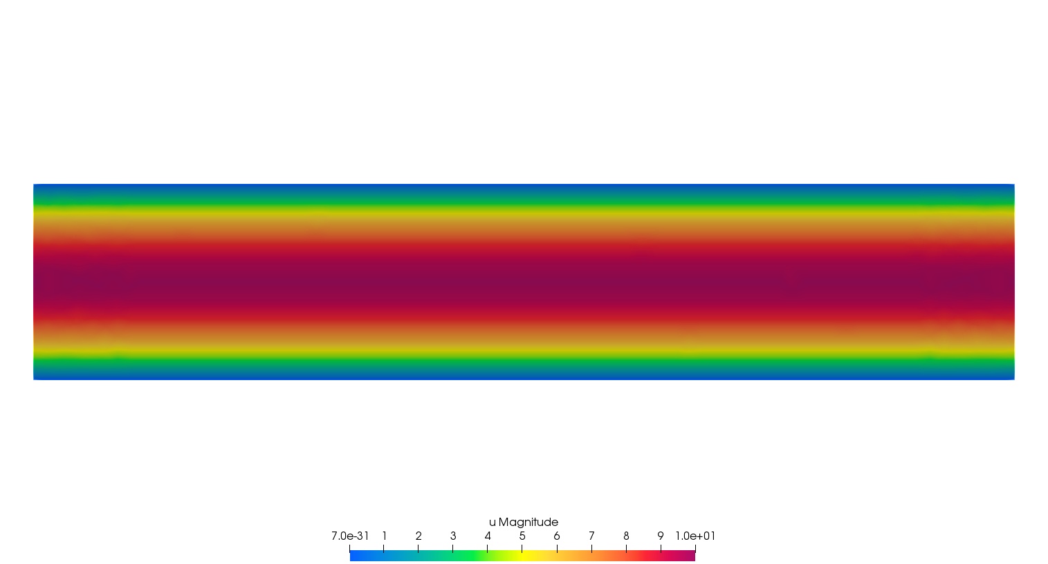
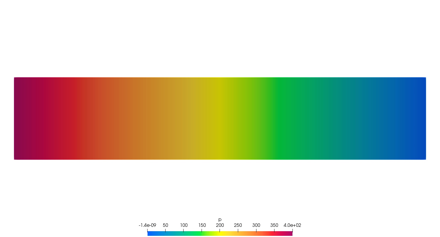
plot(p, cmm="Pressure - i="+i);
plot([ux, uy], cmm="Velocity - i="+i);
}| Result - velocity (top) and pressure (bottom) |
|---|
 |
 |
Authors
Author: Simon Garnotel
From the documentation