
Piezoelectricity
Algorithms for solving the linear piezoelectricity equations
Problem
For time-harmonic case with stress $T$, electric displacement $D$, strain $S$ and electric field $E$, solve for displacement $u$ and potential $\phi$:
$ \displaystyle{
\left{\begin{matrix}
-\omega_0^2\rho_p u_i &=& T_{ij,j}
D_{i,i} &=& 0
\end{matrix} \right.
} $
With:
$
\displaystyle{
\left{\begin{matrix}
T_{ij} = c_{ijkl}^E S_{kl}(u) - e_{kij}E_k(\phi)
D_{i} = e_{ikl} S_{kl}(u) +\epsilon_{ik}^S E_k(\phi)
\end{matrix} \right.
}
$
where $c$ is a 3x3x3x3 elasticy tensor, $e$ - 3x3x3 piezoelectric tensor and $\epsilon$ - 3x3 dielectric matrix
Variational form
The variational form for free vibration (without impedance loads on boundaries) reads as follows:
$
\displaystyle{
\left{\begin{matrix}
-\omega_0^2\int_{\Omega_p}\rho_p v_i u_i \; d\Omega &=& -\int_{\Omega_p} S_{i,j}(v_i) T_{ij}(u_i) \; d\Omega
\int_{\Omega_p} w D_{i,i} \; d\Omega &=& 0
\end{matrix} \right.
}
$
with $v$ and $w$ as test functions.
Algorithms
2D
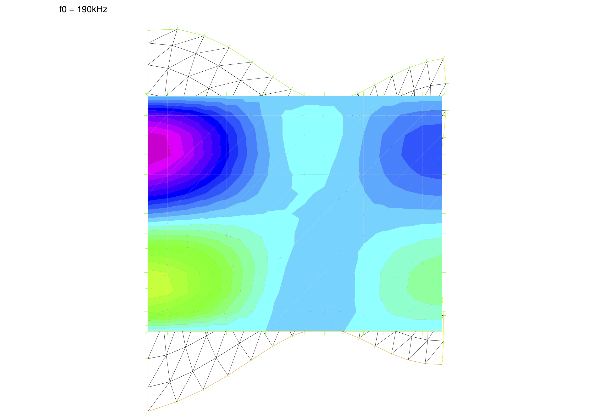
Free vibration of voltage excited piezoelectric circular disc with radius $a$ and thinkness $l$. Due to axisymmetry of the disc shape the analysis is performed in one half of the disc’s cross-section. The bottom (1) and top (3) edges of the rectangular domain represents electrodes and the left edge (4) represents the axis. The analysis is performed in several frequencies located near modal frequencies of the disc. The model uses coefficients of a PZT5A piezoelectric material without losses (real-valued problem) and uses cylindrical coordinates.
// Free vibrations of 2.5cm x 1cm PZT5A cylindrical disc analysed in half of its rectangular cross-section
// Marek Moszynski 30.03.2020

// ------ Variables ------
real[int] ff=[72e3, 73e3, 128e3, 129e3, 156e3, 157e3, 164e3, 165e3, 189e3, 190e3];  // the table of selected frequencies

// ------ Geometry -------
real a=0.025/2, l=0.01;   	                // disc dimensions
int  MM=15, NN=12;				// grid resolution
mesh Sp = square(MM, NN, [a*x, l*y]);           // grid generation
plot(Sp, ps="ff_mesh.eps");                     // plot and save mesh

// ------ Consts -------
real V0=0, V1=1;				// electrode potentials
real rho = 7750;                                // material density
real e31 = -5.4,  e33 = 15.8,  e15 = 12.3,      // piezoelectric consts
     eps11S = 8.1e-9 , eps33S = 7.3e-9,         // dielectric consts
     c11 = 120e9, c12 = 75.2e9, c13 = 75.1e9, c33 = 110e9, c44 = 21.1e9;
						// elastic consts
func C =  [[c11, c12, c13,  0 ,   0  , -e31 ],  // "stiffness" matrix
           [c12, c11, c13,  0 ,   0  , -e31 ],
           [c13, c13, c33,  0 ,   0  , -e33 ],
           [0  , 0  , 0  , c44, -e15,    0  ],
           [0  , 0  , 0  , e15, eps11S,  0  ],
           [e31, e31, e33,  0 ,   0  ,eps33S]];

// ------ Macros --------
macro L(ur,uz,phi) [
 dx(ur), ur/x, dy(uz), dy(ur)+dx(uz), -dx(phi),-dy(phi)] // diff op

for(int ii=0; ii<ff.n; ii++) {                  // for all frequencies
  real f0 = ff[ii], w0 = 2*pi*f0; cout << f0/1e3 << "kHz" << endl;

  // ------ Problem -------
  fespace Vh3(Sp,P1);                           // piecewise linear FE
  Vh3 ur,uz,phi, vr,vz,w;                       // variational variables

  solve Piezo2D([ur,uz,phi],[vr,vz,w])          // variational equation!
   = int2d(Sp)( x * rho*w0^2*[vr,vz]'*[ur,uz] ) // "mass" part
   - int2d(Sp)( x * L(vr,vz,w)'*C*L(ur,uz,phi)) // "stiffness" part
   + on(1, phi=V0)                              // BC: bottom side
   + on(3, phi=V1)                              // BC: top side
   + on(4, ur=0);                               // BC: axis of symmetry

  // -------Plot ----------
  real c2 = 100000;                             // scaling coefficient
  mesh Sp2 = movemesh(Sp,[x+c2*ur, y+c2*uz]);   // deformed mesh
  plot(Sp, Sp2, phi, cmm="f0 = " + f0/1e3 + "kHz", fill=true,
    ps="ff_"+(f0/1e3)+"kHz.eps");               // display and save
}| Deformation warped by a factor 100000 and false coloured potential field inside piezoelectric disc |
|---|
 |
Authors
Author: Marek Moszyński