
Steady Navier-Stokes equations
Newton algorithm to solve the stationary Navier-Stokes equations in 2D.
Problem
Solve:
\[\left\{ \begin{array}{rccl} -\Delta\mathbf{u} + (\mathbf{u}\cdot\nabla) \mathbf{u} + \nabla p &=& 0&\text{ on } \Omega\\ \nabla\cdot\mathbf{u} &=& 0&\text{ on } \Omega\\ \mathbf{u} &=& \mathbf{u}_{\text{in}} &\text{ on } \Gamma_{\text{Inlet}}\\ \mu \nabla \mathbf{u}\mathbf{n} - p\mathbf{n} &=& \mathbf{u}_{\text{in}} &\text{ on } \Gamma_{\text{Outlet}}\\ \end{array} \right.\]Variational form
$ \displaystyle{ \mu\int_{\Omega}{\nabla\mathbf{u}:\nabla\mathbf{v} - p\nabla\cdot\mathbf{v}} - \int_{\partial\Omega}{\left(\nu\frac{\partial\mathbf{u}}{\partial\mathbf{n}}-p\mathbf{n}\right)\cdot\mathbf{v}} = \int_{\Omega}{\mathbf{f}\cdot\mathbf{v}} } $
Algorithms
Start with a guess $\mathbf{u}^k$ and iteratively solve the linearized Navier-Stokes at $(\mathbf{u}^k, p^k)$. \(\left\{ \begin{array}{rccl} -\nu \Delta \mathbf{u}^{k+1} + (\mathbf{u}^k \cdot\nabla)\mathbf{u}^{k+1}+(\mathbf{u}^{k+1} \cdot\nabla)\mathbf{u}^{k} +\nabla p^{k+1} = (\mathbf{u}^k\cdot\nabla)\mathbf{u}^k\\ \nabla\cdot\mathbf{u}^{k+1}=0 \end{array} \right.\)
FreeFEM code
//Parameters
real uMax = 10.;

real Mu = .1; //With smaller of Mu, convection becomes dominant and the Newton method does not converge.

//Mesh
int nn = 10;	//Mesh quality
real L = 5.;	//Pipe length
real D = 1.;	//Pipe height
real R = .2;

int Wall = 1;	//Pipe wall label
int Inlet = 2;	//Pipe inlet label
int Outlet = 3;	//Pipe outlet label

border b1(t=0., 1.){x=L*t; y=0.; label=Wall;};
border b2(t=0., 1.){x=L; y=D*t; label=Outlet;};
border b3(t=0., 1.){x=L-L*t; y=D; label=Wall;};
border b4(t=0., 1.){x=0.; y=D-D*t; label=Inlet;};
border b5(t=1., 0.){x=L/2+2*R*cos(2*pi*t); y=D/2+R*sin(2*pi*t); label=Wall;}; //Empty ellipse : obstacle

int nnL = max(2., L*nn);
int nnD = max(2., D*nn);
int nnDisk = max(2., floor(1.5*2*pi*R*nn));

mesh Th = buildmesh(b1(nnL) + b2(nnD) + b3(nnL) + b4(nnD)+b5(nnDisk));

//Fespace
fespace Uh(Th, [P2, P2]);
Uh [ux, uy], [vx, vy], [ux1, uy1], [dux, duy];

fespace Ph(Th, P1);
Ph p, q, dp;

//Macro
macro Gradient(u) [dx(u), dy(u)] //
macro Divergence(ux, uy) (dx(ux) + dy(uy)) //
macro UgradV(ux,uy,vx,vy) [ [ux,uy]'*[dx(vx),dy(vx)] , [ux,uy]'*[dx(vy),dy(vy)] ]// EOM

real arrns = 1e-9;

macro ns() {
 int n;
 real err=0;
 S;
/* Newton Loop  */
 for(n=0; n< 15; n++) {
   LinNS;
   dux[] = ux1[] - ux[];
   duy[] = uy1[] - uy[];
   err = sqrt(int2d(Th)(Gradient(dux)'*Gradient(dux)+Gradient(duy)'*Gradient(duy))) /
     sqrt(int2d(Th)(Gradient(ux)'*Gradient(ux) + Gradient(uy)'*Gradient(uy)));
   ux[] = ux1[];
   uy[] = uy1[];
   cout << err << " / " << arrns << endl;
   cout.flush;
   if(err < arrns) break;
 }
 /* Newton loop has not converged */
 if(err > arrns) {
   cout << "NS Warning : non convergence : err = " << err << " / eps = " << arrns << endl;
 }

} //EOF

//Function
func uIn = uMax * (1.-(y-D/2.)^2/(D/2.)^2);

//Problem
problem S ([ux, uy, p],[vx, vy, q])
	= int2d(Th)(Mu * (Gradient(ux)' * Gradient(vx)
		+ Gradient(uy)' * Gradient(vy))
		- p * Divergence(vx, vy)
		- Divergence(ux, uy) * q)
	+ on(Inlet, ux=uIn, uy=0.)
	+ on(Wall, ux=0., uy=0.);

problem LinNS([ux1,uy1,dp],[vx,vy,q]) =
     int2d(Th)(Mu*(Gradient(ux1)'*Gradient(vx)
               +   Gradient(uy1)'*Gradient(vy))
	       + UgradV(ux1,uy1, ux, uy)'*[vx,vy]
	       + UgradV(ux,uy,ux1,uy1)'*[vx,vy]
	       - Divergence(ux1,uy1)*q - Divergence(vx,vy)*dp)
     -int2d(Th)(UgradV(ux,uy, ux, uy)'*[vx,vy])
     +on(Inlet, ux1=uIn, uy1=0.)
     +on(Wall, ux1=0.,uy1=0.);


ns;
//Plot
plot(p , ps="pressure.ps", value=1, fill=1);
plot([ux, uy], ps="velocity.ps", value=1, coef=.05);| Result - velocity (top) and pressure (bottom) |
|---|
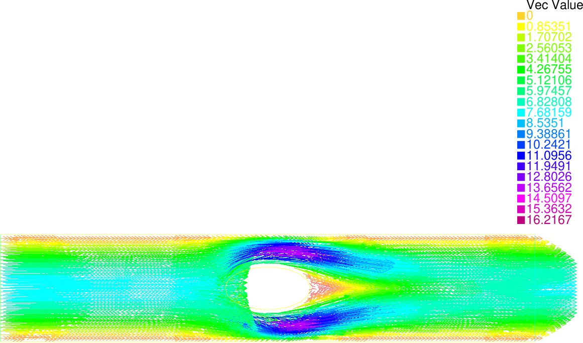 |
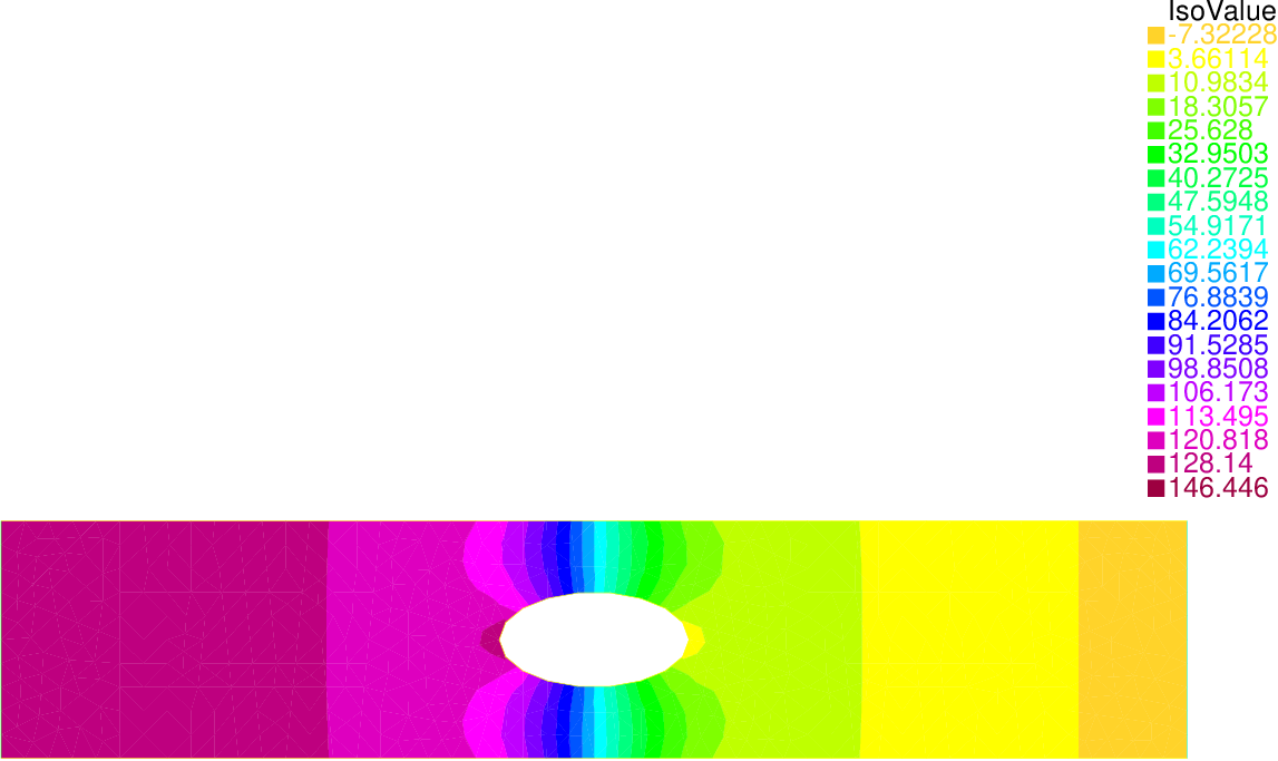 |
Validation
TODO
References
This example is inspired from the official FreeFEM documentation, “Newton Method for the Steady Navier-Stokes equations”.